Pubblichiamo la traduzione del post di Gavin Schmidt su Realclimate, che contiene l’ennesima stroncatura di un articolo pubblicato dal prof. Nicola Scafetta

Pochi giorni fa sulla rivista Geophysical Research Letters (GRL) è comparso un nuovo articolo di Nicola Scafetta (Scafetta, 2022) che ha la pretesa di concludere che i modelli CMIP6 con sensibilità climatica [si veda la nota esplicativa 1 in fondo] media o alta (ECS superiore a 3ºC) non sono coerenti con i recenti cambiamenti osservati della temperatura. Poiché ci sono già stati numerosi articoli su questo argomento, in particolare Tokarska et al (2020), che non sono giunti a tale conclusione, vale la pena cercare di capire da dove proviene il risultato di Scafetta. Sfortunatamente, il risultato sembra emergere da un’errata valutazione di quanto contenuto nell’archivio CMIP6, da un test statistico inappropriato e dall’aver totalmente trascurato l’incertezza osservativa e la variabilità interna.
Insieme a John Kennedy e Gareth Jones del Met Office britannico, ho preparato una breve spiegazione di quello che riteniamo sia stato fatto di sbagliato. I punti principali sono tre:
- Non è stato tenuto conto dell’incertezza nei dati osservati.
- Non si sono considerate le singole simulazioni ma solo le medie di insieme (ensemble mean) dei modelli.
- È stato applicato un test statistico che garantisce l’esclusione di qualsiasi episodio particolare di variabilità interna se il segnale forzato è ben vincolato.
I primi due punti sono illustrati chiaramente da questa figura:
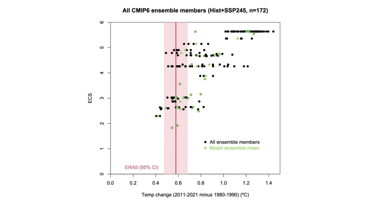
Variazione della temperatura dal 1980-1990 al 2011-2021 nella rianalisi ERA5 e nell’insieme dei CMIP6 in funzione della ECS (Equilibrium Climate Sensitivity, Sensitività del Clima all’Equilibrio) dei modelli.
L’incertezza nell’aumento della temperatura osservata (ERA5) è rappresentata dalla fascia rosa, mentre le singole simulazioni modellistiche sono rappresentate dai punti neri (ce ne sono 172, e quelle dello stesso modello sono sulla stessa linea orizzontale). I triangoli verdi sono la media di insieme (ensemble mean, nota 2) per ciascuno dei 37 modelli (per i modelli che hanno un insieme di un solo membro, il triangolo verde è sovrapposto al punto nero).
Un paio di cose appaiono subito ovvie. In primo luogo, ci sono 3 modelli con una ECS > 3ºC la cui media di insieme è coerente con l’aumento di temperatura di ERA5, entro il margine di incertezza ma, cosa più importante, 49 membri appartenenti agli ensemble di 18 modelli sono compatibili con il risultato di ERA5. Di questi 18 modelli, la metà ha una ECS superiore a 3ºC e contraddice pertanto l’affermazione di Scafetta secondo la quale «tutti i modelli con ECS > 3,0ºC sovrastimano il riscaldamento globale osservato alla superficie».
Per la sua analisi Scafetta usa soltanto la media di insieme per ciascun modello (i triangoli verdi) – nonostante affermi di considerare una singola simulazione – e ignora del tutto l’incertezza di ERA5. Queste sue scelte portano a un risultato fondamentalmente fuorviante. Curiosamente, quando si riferisce ai dati ERA5, cita l’articolo di Huang et al. “Extended Reconstructed Sea Surface Temperature, Version 5 (ERSSTv5)” del 2017 – un set di dati sulla temperatura dell’oceano – invece di Hersbach et al (2020).
Nella seconda parte dell’analisi di Scafetta, l’errore sta nel far riferimento ad un altro errore, di Douglass et al. (2008), peraltro già discusso in Santer et al. (2008). Scafetta sottopone a test la differenza tra le medie di insieme dei modelli (il pattern forzato) e il pattern osservativo esatto (che è la combinazione di un segnale forzato e di una realizzazione della variabilità interna), rispetto all’incertezza del pattern forzato[nota 3]. Questa procedura ha la bizzarra proprietà di garantire, in pratica, l’esclusione dalla significatività statistica (la “rejection”) di tutte le realizzazioni modellistiche di insieme all’aumentare del numero N dei membri dell’insieme stesso (poiché l’incertezza della media diminuisce con, nota 4).
I risultati del test di Scafetta sono quindi inaffidabili.
Che fare?
GRL non accetta commenti sugli articoli pubblicati, una situazione di cui abbiamo già parlato qui. Ha però una procedura per le obiezioni: si segnala il o i problemi alla redazione della rivista che chiede all’autore o agli autori di rispondere. Ricevuta la risposta, il comitato editoriale decide come procedere, il che potrebbe andare dal non fare nulla, al pubblicare una correzione, all’imporre una ritrattazione. Così noi tre abbiamo inviato ai redattori la nota di spiegazione linkata sopra. Staremo a vedere!
Va sottolineato che siamo stati in grado di scrivere la nota così rapidamente poiché sono disponibili e pubblici gli archivi dei dati ERA5, dei valori di ECS per i modelli CMIP6 e del sito Climate Explorer, e per il fatto che errori simili sono stati fatti molte volte in passato.
Che significato avrà tutto ciò?
Come scriviamo nella nota, anche se l’analisi di Scafetta è fallata, ciò non significa che tutti i modelli CMIP6 rappresentino correttamente il periodo storico. E come abbiamo già detto, l’archivio CMIP6 va usato con più attenzione delle versioni precedenti (#NotAllModels, Making predictions with the CMIP6 ensemble). Inoltre, la scarsa performance di uno specifico modello rispetto a questi tipi di osservazioni (rianalisi) potrebbe anche essere dovuta a forzanti non corrette (come gli aerosol, per i quali c’è ancora molta incertezza).
Terremo i lettori al corrente degli sviluppi…
Bibliografia
Douglass D.H., J.R. Christy, B.D. Pearson, and S.F. Singer, “A comparison of tropical temperature trends with model predictions”, International Journal of Climatology, vol. 28, pp. 1693-1701, 2008. http://dx.doi.org/10.1002/joc.1651
Hersbach H., B. Bell, P. Berrisford, S. Hirahara, A. Horányi, J. Muñoz‐Sabater, J. Nicolas, C. Peubey, R. Radu, D. Schepers, A. Simmons, C. Soci, S. Abdalla, X. Abellan, G. Balsamo, P. Bechtold, G. Biavati, J. Bidlot, M. Bonavita, G. Chiara, P. Dahlgren, D. Dee, M. Diamantakis, R. Dragani, J. Flemming, R. Forbes, M. Fuentes, A. Geer, L. Haimberger, S. Healy, R.J. Hogan, E. Hólm, M. Janisková, S. Keeley, P. Laloyaux, P. Lopez, C. Lupu, G. Radnoti, P. Rosnay, I. Rozum, F. Vamborg, S. Villaume, and J. Thépaut, “The ERA5 global reanalysis”, Quarterly Journal of the Royal Meteorological Society, vol. 146, pp. 1999-2049, 2020. http://dx.doi.org/10.1002/qj.3803
Scafetta N., “Advanced Testing of Low, Medium, and High ECS CMIP6 GCM Simulations Versus ERA5‐T2m”, Geophysical Research Letters, vol. 49, 2022. http://dx.doi.org/10.1029/2022GL097716
Tokarska K.B., M.B. Stolpe, S. Sippel, E.M. Fischer, C.J. Smith, F. Lehner, and R. Knutti, “Past warming trend constrains future warming in CMIP6 models”, Science Advances, vol. 6, 2020. http://dx.doi.org/10.1126/sciadv.aaz9549
Note esplicative
[1] La Sensibilità Climatica all’Equilibrio (Equilibrium Climate Sensitivity, ECS) è la variazione di temperatura media globale alla superficie del pianeta che si registra dopo aver raddoppiato la concentrazione di CO2 nell’atmosfera e si è atteso un tempo sufficiente a che il sistema raggiunga di nuovo un ragionevole equilibrio, quindi un tempo di alcuni decenni o secoli. Il Sesto Rapporto di Valutazione dell’IPCC stima che, con un livello alto di confidenza, tale valore sia compreso tra 2,5°C e 4°C, con una best estimate di 3°C.
[2] Il termine “ensemble” da cui “ensemble mean” (insieme, media di insieme) si usa, in generale, ed in questo caso particolare, per descrivere un insieme di realizzazioni simili dello stato e/o dell’evoluzione di una situazione meteorologica o climatica. In questo caso, cioè quello delle simulazioni di scenario CMIP6 (si veda anche https://www.wcrp-climate.org/wgcm-cmip), i vari “ensemble” raggruppano, ognuno, le varie integrazioni modellistiche realizzate con lo stesso modello (anche se in configurazioni più o meno tra loro differenti). Si tratta di 172 integrazioni, raggruppate in 37 “ensemble”, uno per ogni modello specifico (per un elenco dettagliato, si veda la Tabella 1 di Scafetta, 2022.
[3] Anche le singole integrazioni modellistiche (come il pattern osservativo “esatto”) sono la combinazione di un segnale forzato e di una realizzazione della variabilità interna (del modello), ma nella loro media di insieme la variabilità interna si riduce molto, sino a tendere a mediarsi a zero (soprattutto per alti valori della popolazione dell’insieme), lasciando emergere il solo pattern forzato. Da ciò nasce la non confrontabilità statistica delle medie di insieme dei vari modelli con il singolo pattern osservato (ERA5).
[4] Esattamente come eseguire la media (di insieme) di N elementi (integrazioni modellistiche) dell’insieme stesso aiuta a far emergere il pattern forzato (il “segnale”) ripulito dalla variabilità interna (considerata in questo contesto come “rumore”), essa diminuisce anche l’incertezza residua da attribuire al pattern forzato. All’aumentare di N, la variabilità residua (il rumore) tende a zero e quindi tende a zero anche l’incertezza sulla stima del pattern forzato (il segnale). Quindi, all’aumentare di N, la probabilità che pattern forzato e pattern osservato risultino tra loro statisticamente compatibili si riduce enormemente, rendendo molto più probabile la “rejection” del pattern forzato.
Traduzione di Sylvie Coyaud e Stefano Tibaldi


Bello, ho letto in un commento di Realclimate che Scafetta viene definito “the reigning king of Mathturbation”.
https://www.urbandictionary.com/define.php?term=Mathturbation
🙂
http://www.climatemonitor.it/?p=56915
…stroncatura stroncata?
@ Francesco
Direi proprio che la replica di Scafetta è tutt’altro che convincente, sembra ignorare il senso della stroncatura ricevuta; ad ogni modo vediamo quando esce lo scambio su GRL.
Nel frattempo le segnalo questo commento interessante uscito nel post su Realclimate
MS says 1 Apr 2022 at 9:26 AM
A while ago I had reviewed a manuscript by the same author claiming that most of the observed warming is due to urbanisation. I wrote a very careful 4 page review documenting all the flaws of that manuscript in a concise but constructive way. When I received a copy of the decision letter (rejection) I realized that another reviewer had done the same major effort with a 90% overlap on the critical review comments.
A few months later the same paper was published elsewhere. The author simply ignores any constructive feedback and sends the manuscript unchanged to the next journal without even fixing the most obvious flaws. The review process mostly works but if the manuscript is sent to all possible journals over and over and over again, it will at some point slip through the process, which is deeply frustrating.
[Response: Yes – sheer persistence can often win out over quality control. However, while this particular author may be immune to constructive feedback, others can certainly benefit. Consider posting your review on Pubpeer or here? – gavin]
MS says 1 Apr 2022 at 11:04 AM
Here is the paper, more precisely it is about DTR changes:
Scafetta, N. Detection of non‐climatic biases in land surface temperature records by comparing climatic data and their model simulations. Clim Dyn 56, 2959–2982 (2021). https://doi.org/10.1007/s00382-021-05626-x
Here the review for another journal than the one it was ultimately published in. Note that several aspects raised in your comment, e.g. why observations, one realization of internal variability, should not be directly compared to multi-model/multi-member mean has already been explained to the author here in this review and most likely over and over again;
Review: The manuscript submitted by Scaffetta aims at quantifying the effect of urbanization on changes in the diurnal temperature range between 1945-1954 and 2005-2014. The observed difference in the diurnal temperature range is further compared against the CMIP5 multi-model mean difference between the two decades. The author concludes that the CMiP5 multi-model mean overestimates the change in diurnal temperature range and that an increasing urban heat island effect could have contributed to a reduction in diurnal temperature range. The text is clearly written and I spent a lot of time to understand the details of the manuscript and the figures.
Even though the research question per se is interesting I am afraid I have to recommend rejection of the manuscript and I am sorry to say that the manuscript is an example of very poor scientific practice in many respects. The methodology is flawed, the manuscript is full of unsubstantiated claims and speculative statements, the manuscript mixes partly unrelated aspects, the analysis is selective and the citation style includes a lot of self-citation and selective citation, omitting references with conclusions that do not fit the storyline of the manuscript. I detail some of the major issues and I encourage the author to thoroughly and quantitatively address the research question, which I find relevant and interesting.
Diurnal temperature range (DTR): The DTR is controlled by numerous factors many of which the author lists on page 5, third paragraph. However, after listing the factor once, the author completely ignores all other factors that are known to strongly affect the DTR for the rest of the manuscript. Most importantly clouds and atmospheric humidity are well known to be primary drivers of the DTR at subseasonal and interannual time scales as they cool during the day and reduce surface cooling and thereby warm at night. Other factors include tropospheric aerosols and land use changes that are very important but ignored in the analysis. Finally also changes in soil moisture, an important factor that is not listed in the manuscript need to be taken into account. The author argues that urbanization may account for the DTR difference between the two decades. However, this claim is purely based on speculation with zero quantitative analysis to support this claim. The author adds maps of selective land regions and claims that some changes coincide with urbanized areas, whereas it is easy to see that others don’t. There is no quantitatve assessment of the spatial correlation of urbanization and DTR changes nor does the author provide any evidence that the urbanization coincides with the changes in these areas. There is no scientific quantitative evidence to demonstrate that the DTR differences between the two decades are not explained by cloud, atmospheric humidity and soil moisture variations, well documented primary drivers of DTR.
Urban heat island effect: The author further speculates that urbanization may have remote effects and even suggests an interesting scientific hypothesis that in the stable nighttime boundary layer heat is efficiently advected into suburban areas. However, this hypothesis is not tested nor supported by any references yet in the remaining manuscript the hypothesis is suddenly treated as it was a conclusion. In a scientific paper such hypothesis needs to be tested with data and supported by quantitative evidence. The hypothesis that the urban heat island effect would reduce the DTR over such a large radius that it could explain the major blobs shown in the maps of DTR changes is completely at odds with the literature on urban climatology. Why would it be possible to demonstrate such a strong UHI between urban and suburban and rural station if the heat was so efficiently advected over hundreds of kilometers? Again, the hypothesis represents an interesting and relevant research question but needs to be tested quantitatively rather than being speculated about.
Explaining the global average land DTR difference primarily with UHI seems highly implausible simply because the urban land area corresponds to only a very small area fraction of global land. The author would need to provide strong quantitative evidence to demonstrate that an effect over a very small are fraction is the primary driver over global land average changes in DTR.
Comparison against CMIP5 mean: The comparison between observations and the CMIP5 multi-model mean is very poor scientific practice and a flawed approach. The author provides the reason why it is flawed himself in the following statement, which is citing a paper of his, i.e. “… individual model runs appear too random at the required decadal scale. The random “internal variability” tends to cancel out in the ensemble mean”. Likewise, do the observations have random internal variability, which is large for decadal means at the local to regional scale. Or, does the author really want to suggest that all the regional variability in the observations is forced, and even forced by human activity?
If not, the logical consequence is that part (and potentially a large part if the author thinks variability is large) of the difference between observations and any individual model realization is due to random internal variability. There is abundant literature demonstrating that for decadal averages even two realizations of the exact same model forced with the exact same forcing disagree for decadal averages at the grid point scale. Unless the author can demonstrate that the models strongly overestimate unforced random internal variability and all the variations in the observations are forced, the approach he uses is flawed. Instead, an apple-to-apple comparison would either use several single model initial condition large ensembles to test whether the observed differences fall into the range of the different realizations of a model. Likewise, the author could test whether the differences fall within the CMIP5 multi-model ensemble and check whether the observed differences fall into the range of the multi-model ensemble. Only if the observations fall outside the range of models, you can conclude that there is a high chance that the model response is biased.
By construction the multi-model mean averages out most of the unforced internal variability. Thus, it is an artefact of the flawed comparison that the multi-model mean pattern is much smoother than the difference in the observations, which correspond to one individual realization of unforced internal variability. A careful quantitative evaluation would also need to test what fraction of the noisy difference pattern in DTR is due to internal variability e.g. of decadal mean cloud cover.
Given the high level of internal variability it is also unclear why the author analyzes a difference of only two selected decades instead of using as much data as possible to reduce the effect of comparing and trying to interpret patterns of random variability.
The paper also includes incoherent aspects: It is odd that in Fig.10 the author suddenly analyzes mean temperature trend over Greenland when the rest of the paper speculates about urban effects on the DTR. This part is completely unrelated to the rest of the manuscript suddenly uses other selected periods and raises the concern that the author is arbitrarily selecting regions and subperiods.
Finally, the author uses a very selective referencing style including a large fraction of self citation and at the same time ignoring very relevant literature, which previously have shown the DTR changes but have been showing evidence for other drivers.
For instance Sun, X., Ren, G., You, Q., Ren, Y., Xu, W., Xue, X., Zhan, Y., Zhang, S. and Zhang, P., 2019. Global diurnal temperature range (DTR) changes since 1901. Climate dynamics, 52(5-6), pp.3343-3356, https://link.springer.com/content/pdf/10.1007/s00382-018-4329-6.pdf show the same DTR reduction but also demonstrate that part of it is actually likely a reversal of the trend with an increase in DTR in the early 20th century and a reversal in the second half of the 20th century. The first part is another aspect that seriously challenges the speculations on the role of urbanization in this paper.
Likewise, the following two papers provide a thorough documentation of DTR variations in the 20th century. Much of the observed changes are here assessed in a much more thorough and comprehensive way. It is irritating that such directly relevant literature is not referenced in this manuscript.
Thorne, P. W., Donat, M. G., Dunn, R. J. H., Williams, C. N., Alexander, L. V, Caesar, J., et al. (2016a). Reassessing changes in diurnal temperature range: Intercomparison and evaluation of existing global data set estimates. J. Geophys. Res. Atmos. 121, 5138–5158. doi:10.1002/2015JD024584.
Thorne, P. W., Menne, M. J., Williams, C. N., Rennie, J. J., Lawrimore, J. H., Vose, R. S., et al. (2016b). Reassessing changes in diurnal temperature range: A new data set and characterization of data biases. J. Geophys. Res. Atmos.121, 5115–5137. doi:10.1002/2015JD024583
Minor comments:
Page 3: “e.g., through increased shading caused by buildings” How do you know this effect dominates? Buildings may shade during the day but they also reduced longwave outgoing radiation at night by reducing the skyview factor (i.e. longwave trapping).
Page 4: “because the heat produced by the urban areas can actually be transported from one region to the surrounding one by wind and radiation.” Can you provide quantitative evidence that radiation plays a relevant role in the horizontal transport of heat in this case?
Page 4: PBL and UHI: An interesting hypothesis, please provide quantitative analysis of the lateral transport of nighttime urban heat to support the hypothesis.
Page 5: Why would you limit the analysis to a difference of means over only a decade and thereby discard all the data in between? The regional pattern analysis is likely affected by high random internal variability.
Page 5: “poorly model the ocean and atmospheric circulation”: This is a simplistic general statement that is not supported by a substantial fraction of the scientific literature and a biased and opinionated representation of the scientific literature.
Page 5: “non-climatic biases which could also be involved. For example, changes in local microclimate (Fall et al., 2011)” Why do you refer to change in local microclimate as a “bias”?
Page 6: “The records were interpolated to fit a 0.5°x0.5° grid.” Why do you increase the grid resolution to a higher resolution rather than coarse-grid everything to the lowest common resolution, which is common practice?
Fig.3 and Fig.4: Do you mask the models to the observational grid to allow for a thorough comparison?
Page 8: “Figure 6 shows that the CMIP5 GCM temperature simulations produce, as expected, nearly spatially homogeneous results. These are characterized by a much less regional variability spanning between -0.3 °C and 0.5 °C.” This result is an artefact of the flawed apple-to-orange comparison. In the models you smooth out random internal variability, in the observations may explain a substantial fraction of the pattern.
Page 8 and 9: Can you provide any quantitative evidence that the differences discussed here at the local scale are really forced and not just random internal variability?
Page 10: “The figure confirms that the most populated regions characterized also with a high concentration of urban centers are often also the ones with the largest divergence between the warming observed in Tmin and Tmax.” Provide quantitative evidence rather than speculations. How about all the changes over Siberia and many other non-urbanized areas in Fig.5?
Page 11: As stated above the mean trend analysis over Greenland is completely unrelated to the rest of the paper. It is very odd to read that “Greenland should be one of the few regions of the world that is mostly free of any bias.”. How many stations are available over Greenland? It is likely one of the regions with the poorest spatial coverage globally.
Fig.3 top right: I think the red label should read Tmax.
Fig.8 Why is there suddenly hardly any variability in the CRU data set here? Have you applied any temporal smoothing here?
@ Stefano
Guardi, io non sono uno scienziato (neanche lei peraltro) e non sono quindi in grado di scendere nel merito della vicenda.
Tuttavia, essendo invece abituato a valutare il linguaggio delle persone, al di là di quel che concretamente scrivono, posso dirle che sottotitolare un post di argomento scientifico con l’espressione “ennesima stroncatura di un articolo…” significa squalificare inevitabilmente la pretesa scientificità del testo.
Cari saluti
F.
@ Francesco
per vedere se lavoro o no in ambito scientifico può vedere le mie pubblicazioni, le trova facilmente nei siti specializzati.
In ambio scientifico è normale definire stroncatura una critica come quella mostrata nel post; può non piacerle ma è così.